One of the most interesting upcoming areas of football analytics is Expected Threat or (xT). We’ve slowly become used to analytics data like xG(Expected Goals) and xA(Expected Assists) which allow us to predict and evaluate player performance.
What Is Expected Threat?
Expected Threat or xT evaluates the probability of scoring a goal based on the position of the player on the pitch and his probability of either shooting, passing or dribbling. So we evaluate an action i.e shooting, passing or dribbling, and how that action changes the probability of scoring.
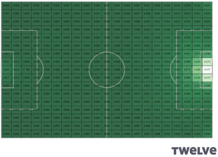
To do that, every section of the football pitch is divided into quadrants and is assigned a value based on the probability of scoring based on that particular position on the pitch.
Expected threat (xT) for different parts of the pitch. These show the probability of a goal being scored given that a team has possession at this point of the pitch. Created by Jernej Fllsar at Twelve.
So of course areas inside the box have a higher probability of scoring as compared to midfield or the wings.
As David Sumpter, author of the book Soccermatics writes:
“If a player makes a pass which moves the ball from a place where it is unlikely for their team to score, to a place where they are more likely to score, then they have increased the xT in favour of their team. In general, the nearer you get the ball to the goal the more likely your team is to score (although if you look carefully passes back to the goalkeeper are also valuable).”
The Sarah Rudd Model
Although it seems like a newer revelation and concept, it was in fact invented by a woman named Sarah Rudd in 2011.
Rudd made the earliest xT model based on Markov Chains(As shown in the figure below)

To make this prediction, because football is so random, we can only estimate the probability within ideally 1, 5 or 10 seconds. This is because there are so many possibilities beyond 10 seconds like in a minute or more.
So in Rudd’s model, this is 5 seconds into the future where scoring a goal from that position in the center outside the box marked as M is 5%, going to the wing marked as position W is 10%, playing the ball into the box marked as B is 20%, losing the ball marked as L is 40%, and lastly the probability of it staying in midfield is 25%
This sets up what is called a Markov Chain of probability, which basically means if the ball is moved out to the wing, at position W, you then start the whole analysis from position W, and then if it’s moved into the box at B you then begin from that point and so on.
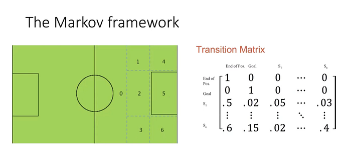
To further explain Rudd’s model, she used a Transition Matrix.

Rudd marked the positions on the pitch to divide them into seven areas, as shown in the figure above. 0 being the area where not much is likely to happen, 2 just outside the box, 1 and 3 on either side outside the box, 4 and 6 on the flanks and 5 inside the box.
She then used a Transition Matrix which looks at the probability of going between these areas like 2 to 5 or 2 to 6 or 6 to 5 or 4 to 5 etc, with the final transition being a goal or the end of possession(marked as 1 in the above matrix) which she estimated using Opta data to parameterize the model.
She could then evaluate players based on their actions that lead to a goal based on their xT.

So if player 1 moves the ball to player 2 in another zone, as shown in the above figure and the probability of scoring reduces from 0.25 to 0.17 player 1 gets a negative value of -0.08. But if player 2 makes a pass to player 3 increasing the probability of scoring from 0.17 to 0.28 he gets a positive +0.11 value. And finally if player 3 scores a goal, he gets a value of +0.72.
This was the basic model invented by Rudd.
Rudd gave a talk about this model all the way back in 2011, and was signed by Arsenal as the head of analytics after it and continues working there.
Karun Singh’s Model
Karun Singh, an analyst from the US, had another model, which he dubbed as xT and posted in the public arena on his blog in 2018.
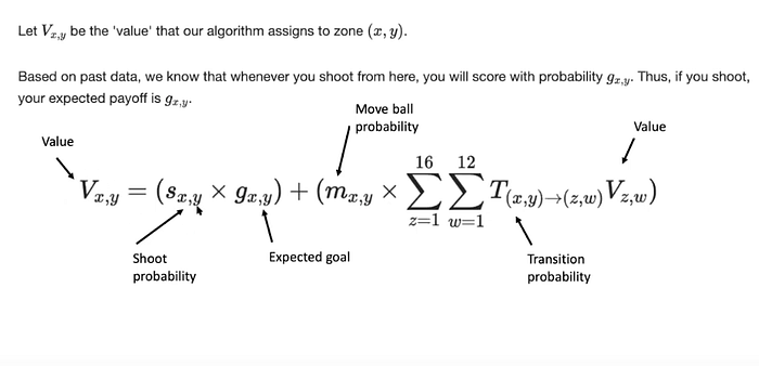
Singh’s model broke the pitch into finer granularity and he hypothesized an equation to calculate it.
There’s some math involved in this which we will break down.

As shown in the figure above, V(x,y) is the value of each quadrant or zone (x,y) the x-axis being the length of the pitch from goal to goal as a 2D map and y being the y-axis or the breadth of the pitch in a 2D map.
s(x,y) is the probability of a shot and g(x,y) is the probability of a goal.
So V(x,y) = Either a shot or goal or a shot probability multiplied by a goal probability i.e. s(x,y) X g(x,y) while m(x,y) is the probability of moving the ball and the transition probability T from a point i.e T (x,y) to a new position (z,w). The latter of which are passes or dribbles. And the value at the next new position i.e. V(z,w).
So V(x,y) gives the value of the old area where the ball was and V(z,w) gives the value of the new area where the ball goes, and then this repeats.
All the data for these parameters are available on Opta, Statsbomb or other data companies and you then solve for the values or V.
So to make it sound a bit catchy, V(x,y) was dubbed as xT(x,y) or Expected Threat by Karun Singh in 2018.
You can find interactive dynamic visual charts (although they’re made in 2018) for xT for each Premier League team that season.
Karun has done a fantastic job theorizing and coining the term xT.
You can check Singh’s blog post by clicking the following link: https://karun.in/blog/expected-threat.html
There are far more advanced ways of calculating xT that have evolved since Rudd’s talk in 2011. But, this is a basic & simplified explanation of xT.


