The Ultimate xG Resource – What Is xG? Understanding xG, Misconceptions, Variance & Use Of xG

When it comes to analysing football matches, teams, and players, xG plays a significant role in estimating team performance based on probability. xG was first introduced by Opta’s Sam Green in 2012 and has expanded going into much more detail as a tool of analysis in the last decade.

Nowadays, xG has become a vital point of discussion, and analysis. However, it is a cause for a lot of debate, arguments, and questions.

Although results are the most important, in the modern era, football enthusiasts immediately check their team’s xG after a game and decide which team had performed better. However, there is significantly more depth to xG and the way it can be interpreted and used as a tool of analysis.

In this article, we set the record straight and dive right into the topic and explain xG in detail and in as easy terms as possible.

Also read: Premier League xG v GF: How Clinical Are The Prem Teams?

What Is xG?

Simply put, xG is defined as the number of goals a team could have expected to score based on historic data and events leading up to the goal or in a simpler way, the probability of a shot leading to a goal based on certain parameters.

There have been many instances where a team performed better than the other but didn’t win the game. If you’re wondering if your team had more chances, more possession, and more shots on goal, but didn’t win and want to quantify it, in comes xG.

By quantifying chances, we can come to a conclusion about how to analyse and prepare teams for fixtures ahead and xG serves as a tool of measuring performance.

How Is xG Calculated?

When we watch a football game, we can assess which instances are more likely to result in a goal or not, like shooting from closer to the goal or inside the six-yard box as compared to shooting from outside the box, or perhaps a one v one situation with a defender or a goalkeeper, or if the angle was favourable or difficult to score from.

These are assessments we make intuitively. xG on the other hand uses situations like these in their data sets.

Football data companies like StatsBomb, Opta, Understat, and a wide range of others calculate xG based on models.

What these companies do is take databases of historic data of thousands of shots and use data points like the type of shot, the relative position on the pitch and where all the players were on the pitch, the angle of the shot, player’s body position, the relative defender’s position, the distance to the goal, the speed, and type of the pass, etc.

This data is fed into complex machine learning algorithms which calculate probabilities for a particular shot. The probabilities of all shots attempted in a game by a team are then added. That gives you the xG for a team.

The models use historical data of thousands of shots to assign a value of the probability of a goal on a scale between the values 0 and 1.

An xG of 1 is a definite goal while an xG of 0 is a definite miss.

The machine learning algorithm then assigns xG values based on all the data parameters.

The Math Behind Calculating xG For A Single Offensive Play

This is the example of how to calculate xG for a single offensive play explained on the free football data website FBref. (We love the work they’re doing)

To explain the calculation they use the reference of a match between Schalke & Nurnberg in the Bundesliga in the 2018 season. The match ended 5-2 with Schalke winning. But the example uses one of Nürnberg’s goals.

In the 78th minute, Nürnberg attempted three shots which ultimately led to a goal.

1) Hanno Behrens attempts a shot that is saved

2) He is able to take a second shot as the ball is deflected off the defender.

3) The second shot hits the woodwork

4)Adam Zreľák gets to the rebound to easily tap it in.

“According to StatsBomb’s expected goals model:

• Behrens’ first shot with the goalkeeper in his way = .37 xG
• Behrens’ second shot with the goalkeeper out of position but a defender in the way = .68 xG
• Zreľák’s shot with an open net = .81 xG

The sum of these three shots is 1.86 expected goals, even though it is impossible to score more than one goal in a single move. To solve this problem, we find the probability that the defending team does not allow a goal in this possession. In this case, the calculation is:

(1 - .37) x (1 - .68) x (1 - .81) = .0383 or a 3.83% probability that Schalke does not allow a goal.

To find Nürnberg’s xG, we simply subtract that probability from 1:

1 - .0383 = .9617 xG

In other words, we estimate that an average team in a similar situation would be expected to score a goal 96.17% of the time.

We use a similar method when calculating xG for individual players. Adam Zreľák receives .81 xG from his single shot while Hanno Behrens receives:

1 - (1 - .37) x (1 - .68) = .7984 xG

This shows why a team or player’s total xG may not equal the sum of the xG from their shots and why a team’s total xG may not equal the sum of the xG from their players.”

(We hope the math wasn’t too complicated)

Misconceptions About xG

A common misconception about xG is that we can “expect” the teams or players to match their exact xG. Yes, they do either overperform, nearly match or underperform their xG. However, “expected goals” is derived from “expected value” in mathematics which is only the “likelihood” of an event occurring.

For example, the probability of a coin toss is 50% for heads or tails or a 0.5 probability for the coin landing on heads and tails. That doesn’t mean you get heads or tails in 50% of your coin tosses or half of your tosses will be heads or tails. But rather, these values could regress to 50% over thousands of tosses.

It’s the same with xG.

The xG of teams and players is just a framework to measure their performance i.e. a barometer to measure performance and not actually expecting them to score those many goals.

Also, another common misconception is that xG determines who should have won the game, which a lot of football followers & fans often jump to conclusions about post-game.

Basically, a team with a higher xG in a game might not win the game, and further, a higher xG doesn’t mean that they should have won the game. As mentioned earlier, xG just measures chance quality and not the expected final result of a particular game.

And for example, if a team gets an early lead, they might sit back and defend and not want to create more chances which means they will underperform their xG. The same logic can be applied to teams looking to close out a game as a draw if they’re looking to scrap a point from the game, they’ll underperform their xG as well.

In these areas, xG doesn’t represent the view of the entire game, but rather just an estimate of the team’s performance in front of goal based on historical data of shots from those positions and other in-depth parameters.

Variance in xG

Qualitative Variance

Variance in xG can occur in a few situations. Qualitatively and quantitatively.

Qualitatively, for example, considering the actual player before comparing him to his performances vs xG. For someone like even Cristiano Ronaldo, for instance has underperformed his xG for the best part of 7 seasons now.

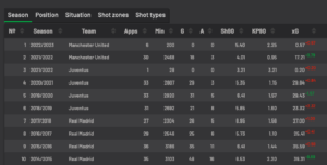
Looking at his xG over the years, Ronaldo has overperformed his xG only twice and nearly matched it once. Yes, his actual goals scored is close to his xG but he has underperformed, by fine margins, but he has. Does that mean he’s a bad player? No.

He takes more shots and his xG is something he rarely has matched in the last 7 seasons, but as a player, he’s perhaps the greatest to have graced the game.

It’s similar with other elite strikers like Robert Lewandowski and Karim Benzema. They have also underperformed their xG.

On the other hand, there are players that regularly overperform their xG, like Harry Kane, Lionel Messi, Kevin De Bruyne, and Heung min-Son.

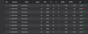
Having an xG of 0.5 is different for an average player as compared to an elite finisher like Kane, Messi, or Son.

That’s what is the qualitative nature of xG. You have to take the player into account.

Overperforming xG doesn’t mean they’re good players, rather it means that they’re the best finishers. Or in other words, because they overperform their xG they’re the best players out of the database of all players to score from a particular position or situation or the best at putting away chances.

It’s football, and despite analytics increasing in leaps and bounds, and efforts to quantify the game and predict things, it’s still a game where anything can happen in a second.

Quantitative Variance

However, there are certain quantifiable instances where the data just doesn’t lie.

This is quantifiable variance.

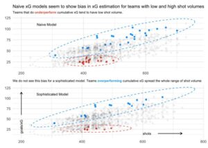
Consider two teams with around the same xG. According to the data and running thirty thousand instances of them in an xG model, the team with lesser shots is more likely to win.

In this case, we will look at two teams with an xG of 2.

Suppose one team has 4 0.5 xG chances vs one team with 12 0.167 xG chances and they play each other thirty thousand times, the team with 4 0.5 xG chances will always have more wins. This is primarily because of variance.

So essentially, the lower the xG of the shot, and the more of them there are, the more variance it will result in.

The team with 4 0.5 xG chances has a variance of 1, while the team with the 12 0.167 chances has a variance of 1.29.
The lower the variance, the better the team’s chances are of winning.

Both still have an xG of 2, but the team with lesser chances, is more likely to win. This is purely based on probability and data and it gives an interesting picture when running the data of instances of games where this variance occurs.

Variance, is, however, a stat that needs to be computed and there aren’t many platforms providing stats for variance. But as football analytics develops further we could get access to this quantitative way of analysing games.

Uses Of xG

Again coming back to the uses of xG as mentioned on the excellent FBref.

“xG has many uses. Some examples are:

• Comparing xG to actual goals scored can indicate a player’s shooting ability or luck. A player who consistently scores more goals than their total xG probably has an above average shooting/finishing ability.
• A team’s xG difference (xG minus xG allowed) can indicate how a team should be performing. A negative goal difference but a positive xG difference might indicate a team has experienced poor luck or has below average finishing ability.
• xG can be used to assess a team’s abilities in various situations, such as open play, from a free kick, corner kick, etc. For example, a team that has allowed more goals from free kicks than their xGA from free kicks is probably below average at defending these set pieces.
• A team’s xGA (xG allowed) can indicate a team’s ability to prevent scoring chances. A team that limits their opponent’s shots and more importantly, limits their ability to take high probability shots will have a lower xGA.”

Takeaways And What xG Models Have Revealed

Statsbomb, who also calculate xG have identified four key learnings that all their xG models have revealed.

As mentioned on their website, here are some of the important takeaways. These are also perhaps a bit intuitive and anybody with enough knowledge about the game can explain and understand these learnings.

Central Shots Are The Best

Shots from the central part of the box are more valuable than shots from tighter angles and are more likely to result in goals. This perhaps can be assessed intuitively as well, because you have either side to aim at and score a goal. And tighter angles do result in lower xG.

Crosses Are Difficult To Convert

The traditional way and ploy of wingers and fullbacks running to the touchline and crossing balls into the box is a useful tactic for many managers, however, the data shows that crosses are harder to convert as compared to through balls, ground passes, and shots after successful dribbles.

Shot Over Header But Not For Set Pieces

From the same positions, shots are more likely to result in a goal as compared to headers. This is pretty obvious. However, this is not the case for set pieces, but again it depends on the kind of set piece. Like for corners and free kicks from a longer distance, headers are more likely to result in goals. This is again pretty intuitive, but the data agrees on it.

Shot Quality & Location Is Key

After running the models for large sample sizes and data sets, it reveals that most players are average when it comes to finishing. However, there are stand out players who have a better finishing ability than the large set of average players. In the end, goal scoring and finishing ability is not so much scoring more chances at a higher rate but rather taking shots and finishing from more valuable locations on the pitch.

Conclusion

Football analytics and xG have evolved over the years since their inception. Now we have more data-centric decisions in scouting, coaching, transfers, management, and all aspects of football, that translate to decisions on the pitch and the very fabric of how football is played.

Football is a simple game. But data and algorithms that give us in-depth insight into how the game is played certainly helps in the broader perspective and for the future of the game.

The future will surely see more interesting evolutions of data-driven stats and complex models as technology progresses that explore all aspects of football and the ideas to quantify it.

The xG revolution began a decade ago and is now widely used in television and punditry and is slowly becoming more commonplace when it comes to being accepted and understood by football fans around the world. It’s exciting to see what further evolutions xG take shape in

It’s certain that the future is coming and it will empower the coming generations to explore various facets of the beautiful game.

If you liked this article, you can also read our exploration of Expected Threat or xT by clicking the link below!

Also read: Explaining Expected Threat (xT) In Football Analytics Using Markov Models & Its History